Advanced Features
ATHLETICS has 3 main advanced features: the abilty to create phase, Lorentz and stray field line profiles; the abiltiy to use user defined inputs, created in IGOR Pro, instead of micromagnetic simulation outputs; and the abilty to view many heights above the sample when scanning the out-of-plane stray field.
Line Profiles
To create a line profile of a phase, Lorentz contrast or stray field image, click on the ‘Image’ tab and select “Image Line Profile’.
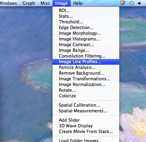
Select the ‘Image Line Profile’ option from the ‘Image’ tab
This then automatically adds a horizontal blue line to the top graph and produces the corresponding line profile along that line. This line can be changed to vertical, or horizontal or vertical freehand using the tab in the top left of the box.

A horizontal blue line and the corresponding line profile are created. This can be changed using the tab in the top left
If horizontal or vertical is chosen then the blue line can be clicked and dragged to produce line profiles along the new lines. If horizontal or vertical freehand are chosen then a red line appears and the points of the line can be moved by using the ‘start editing path’ button in the top left, and corresponding line profiles are created.

Selecting horizontal or vertical freehand allows for user defined line profiles
To move the line profile to a different graph, click on the new graph and then click on the line profile window again and it will update to the new graph and add a line to this graph. To save the graph go to the ‘File’ tab and select ‘Save Graphics….’.The example above is for a stray field graph but this is equally applicable to phase or Lorentz contrast images.
User defined inputs
It is possible to define the x and y components of the magnetisation in IGOR Pro and use these as starting points to simulate holography, Lorentz and stray field images. This may require specific dimensions and set up so it is advised that the authors are emailed so that the script can be adjusted accordingly. Firstly, 2 matrices of the desired size need to be made. Note that the number of cells in each direction is the dimension of that direction divided by the resolution. This can be done by typing ‘ make/o/n=(xdim,ydim) xmag,ymag ‘ into the command window, where xdim and ydim are the number of cells in the x and y direction respectively. A function can then be assigned to each matrix to produce the desired microstructure. The example below is a simple single magnetic domain wall where the moment only has y component that is positive on one side of the domain wall and negative on the other. The profile in the wall has the tanh form expected.
The y component of the magnetisation changing between 1 and -1 across the wall
The x component of the magnetisation, which in this example is zero through out the simulation
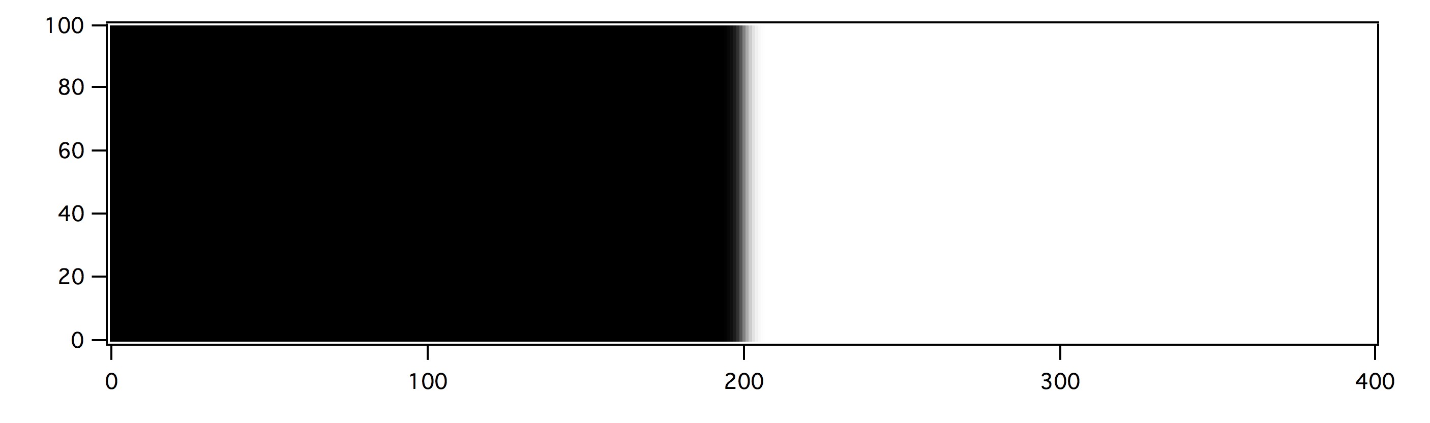
From these inputs (and after modifying the script slightly so extra area around the sample wasn’t included) Lorentz contrast images are produced that can be quantitatively compared to experimental results with very good agreement. The details of the fringes in the Lorentz contrast are reporoduced by ATHLETICS and compare well with experiments.
Lorentz contrast image of the magnetic domain wall sowning fringes of specific amplitude and spacing

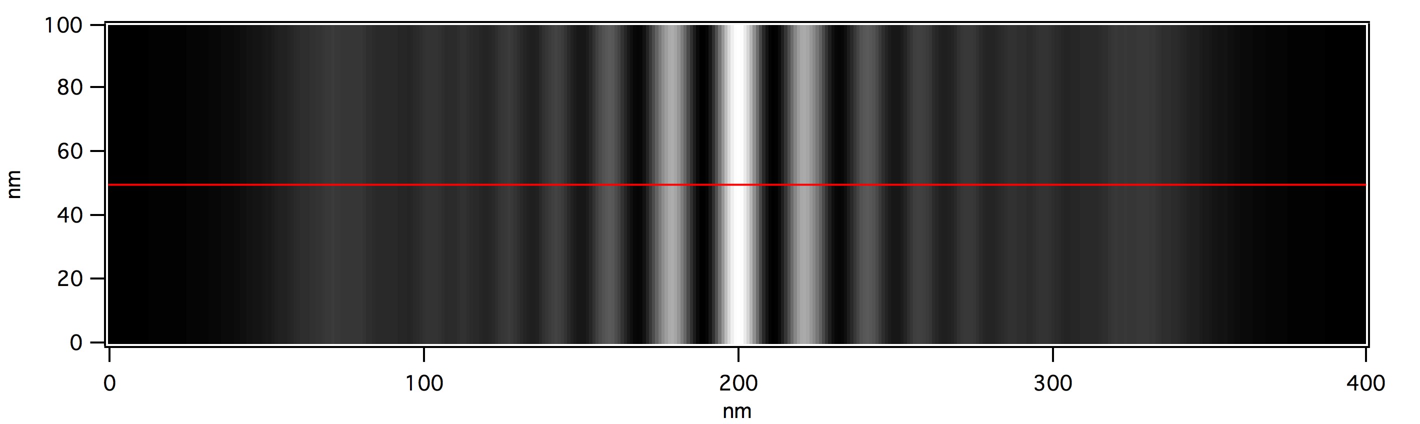
Line profile across the red line on the Lorentz image showing the fringes
It is also possible to take this idea further and create full microstrucutres in IGOR Pro. This requires a knowledge of IGOR Pro, and the authors are happy to give instructions and advice on how to do this. Below are some examples of inputs and there results for full microstructures generated in IGOR Pro to show the kind of images that can be created.

x component of the magnetisation for a user defined function in IGOR Pro
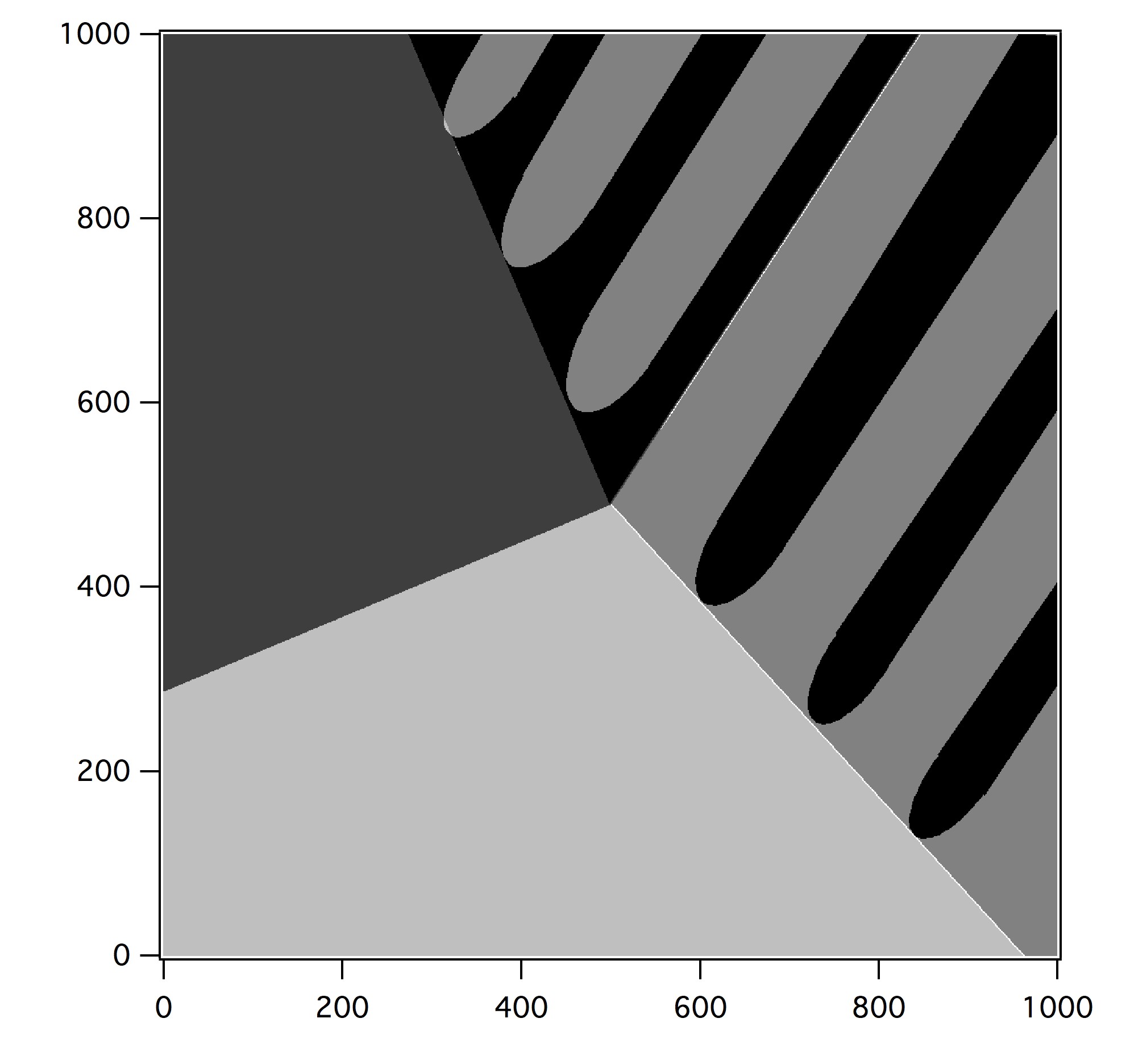
y component of the magnetisation for a user defined function in IGOR Pro

Holography Image created from the user defined microstructure
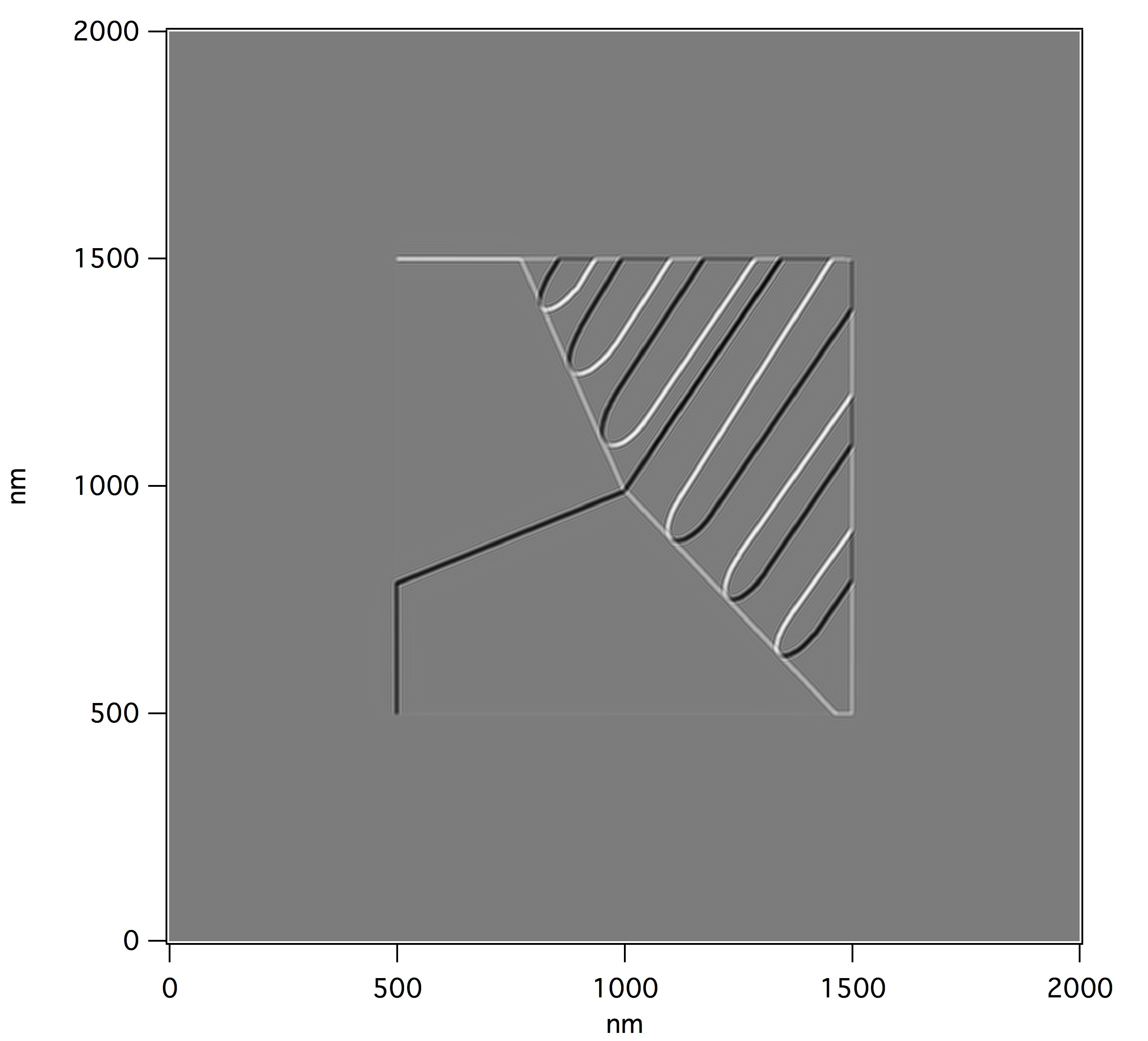
Lorentz Image created from the user defined microstructure
Variable heights above the sample when creating out-of-plane stray field images
It is possible to look at various heights above the sample when producing out-of-plane stray field images. This can be done by selecting the ‘3D Wave Display’ from the ‘Image’ tab in IGOR Pro.
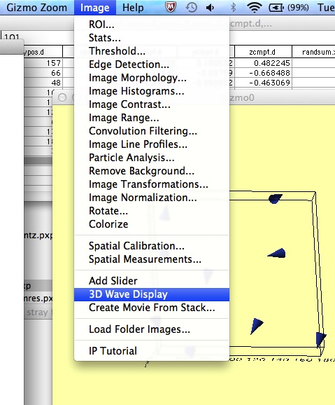
Select ‘3D Wave Display’ from the ‘Image’ tab
From the menu choose ‘Bkz_IFFT’ and click on the OK button on the left.
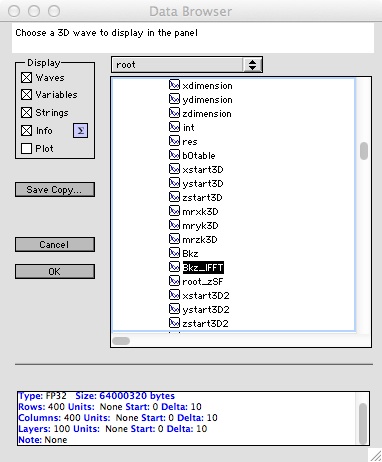
Select ‘Bkz_IFFT’ and click OK
This will produce a window that allows layers to be chosen in all 3 dimensions. The left hand window is the z dimension and changing the slider above this window scans the different layers of the image, so the change in stray field with distance from the sample can be seen. The layer can be saved by clicking the ‘Save Slice’ button. The Z_stray_field macro can produce this layer as the output image by inputting the desired layer as the height above the sample. The slider should be set so the plane being viewed is always above or below the sample and not in it – the sample is at the center of the 3D matrix so only look at greater than half of the z dimension above the center of the matrix.
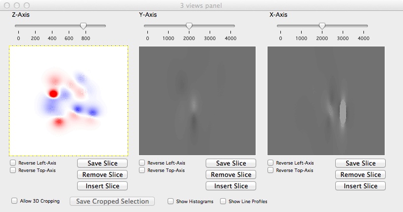
The left window shows the z plane corresponding to the slider above it