Data Visualisation – Paraview
https://www.paraview.org/download/
Paraview is an open source, data visualisation software, ideal for viewing data before meshing, after meshing and after micromagnetic simulations. Paraview is also useful as it can be used to convert image stack data into a surface mesh, whilst retaining the aspect ratios of the data. Paraview itself contains significant user resources, which can be found under the ‘help’ tab.
Opening and Viewing Data
Image Stacks
![]()
Opening Data
Opening image stack data is done using the ‘Open…’ function, which can be accessed via the file tab, the Open… icon or by Ctrl+O. This opens the ‘Open…’ window, as shown in Fig.1.
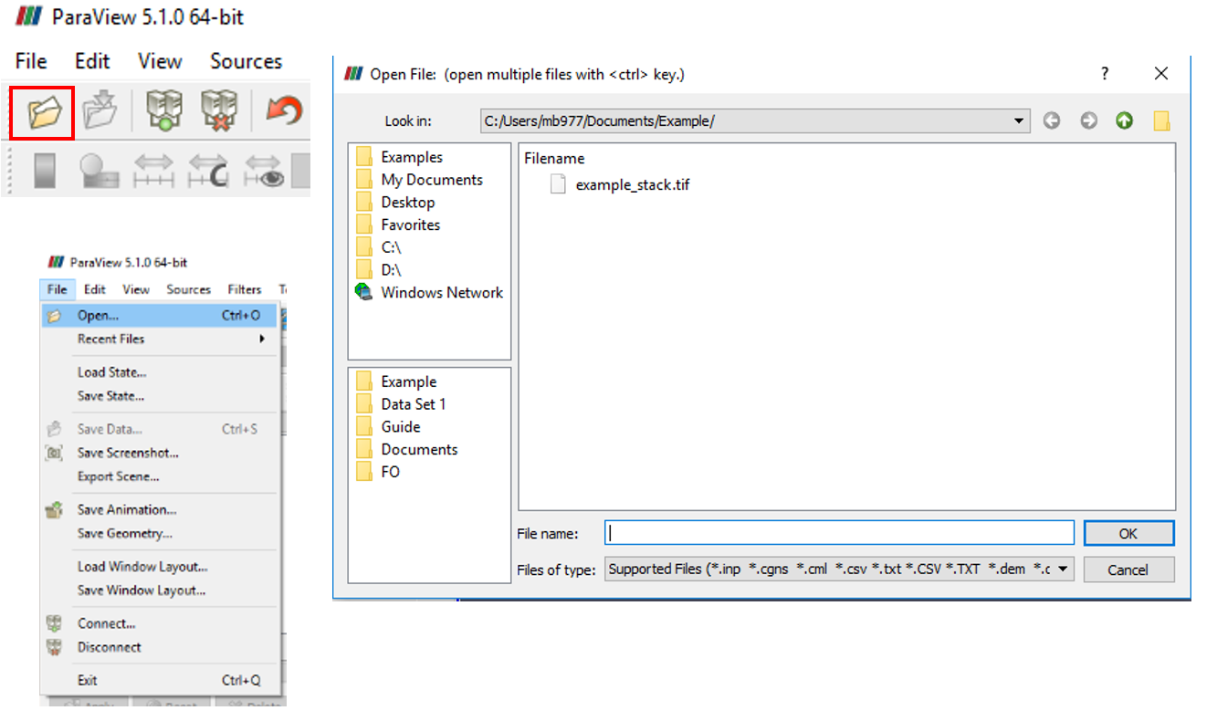
Fig.1 shows the varying ways data can be opened in Paraview
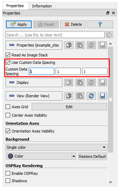
Fig.2 shows the Custom Data Spacing option, highlighted in red, which is used to define the x, y and z dimensions of each voxel
Once the data has been loaded, but before it can be visualised, the voxel size (x, y and z dimensions) needs to be defined in the Properties tab, located in the bottom left of the window. Using the ‘Use Custom Data Spacing’, shown in Fig.2, the x, y and z dimensions of each voxel are defined. The dimensions should be defined in micrometres, since these are the units used in MERRILL. Once this has been applied, the data can then be visualised.
Visualising a Volume
By default, Paraview will display only the outline of the bounding box of the data, this can be change by selecting ‘Volume’ in the ‘Representation’ tab. This can be found at the top of the window, as shown in Fig.3, or in the Display tab, found beneath the custom data spacing option in the Properties tab, shown in Fig.4.
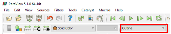
Fig.3 shows the Representation tab, highlighted in red
![]()
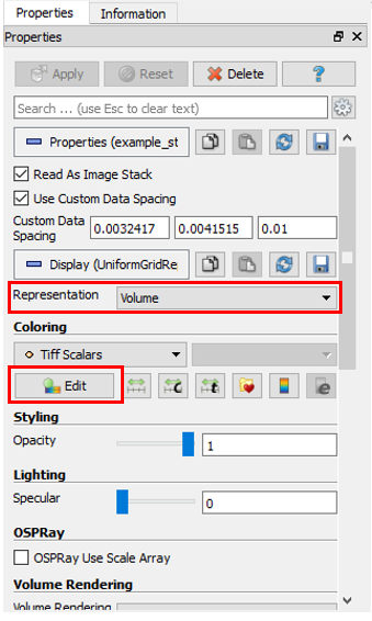
Fig.4 shows the Properties tab, found in the bottom right of the window, with the Representation tab and Colour Edit tab highlighted in red
This will display the data by assigning colours, initially on a scale from blue to red, to the voxels depending on their value. The colour scale of this visualisation can be controlled using the ‘Edit’ function, found beneath the Representation tab in the Properties, as shown in Fig.4.

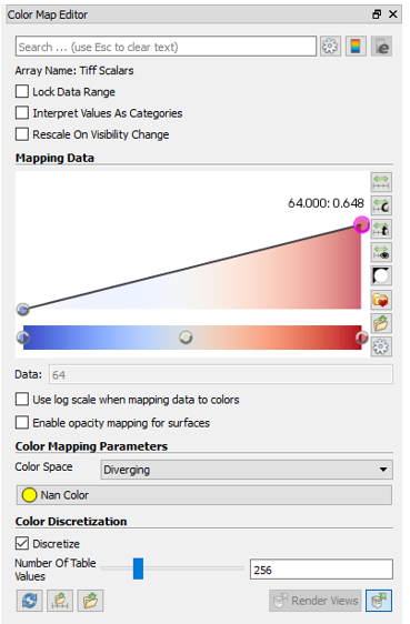
Fig.5 shows the Colour Map Editor, here the colour and scaling of the data can be controlled
Volumes can be visualised by editing the ‘Mapping Data’ tab shown in Fig.5 to change the colour and scaling. For example, the particle shown in Fig.6 was created by increasing the scaling of the low value voxels and decreasing the high value voxels to zero, since the data ranged from 16-64, with the particle defined by the low value voxels.
![]()

Fig.6 shows the example particle displayed as a volume
Visualising a Surface

Fig.7 shows the example particle viewed as a contoured surface
Data can also be visualised as a surface using the ‘Contour’ function, which can be used using either the Filters->Common tab or the ‘Contour’ icon as shown in Fig.8. The contour is taken at a user defined voxel value, which is set in the Properties tab, also shown in Fig.8. The resulting surface is shown in Fig.7.
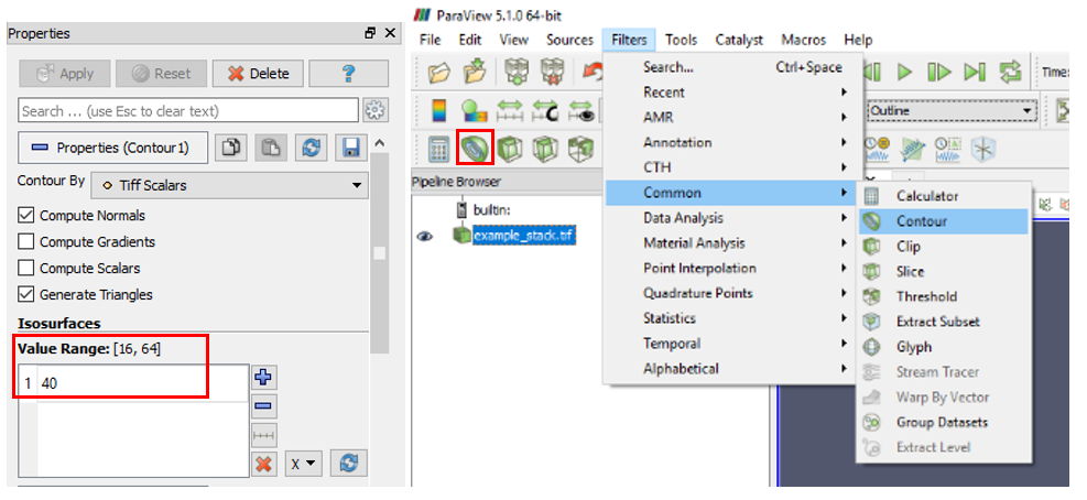
Fig.8 shows the user defined threshold for creating the surface (left) and the two ways of taking a contour (right), the icon, highlighted in red, and the function as found in the Filters tab
Smoothing a Surface
Surfaces created from image stack data is often stepped, as in Fig.7. Smoothing can be done in Paraview using the ‘Smooth’ function, which can be found in the Filters>Alphabetical tab, as shown in Fig.9.
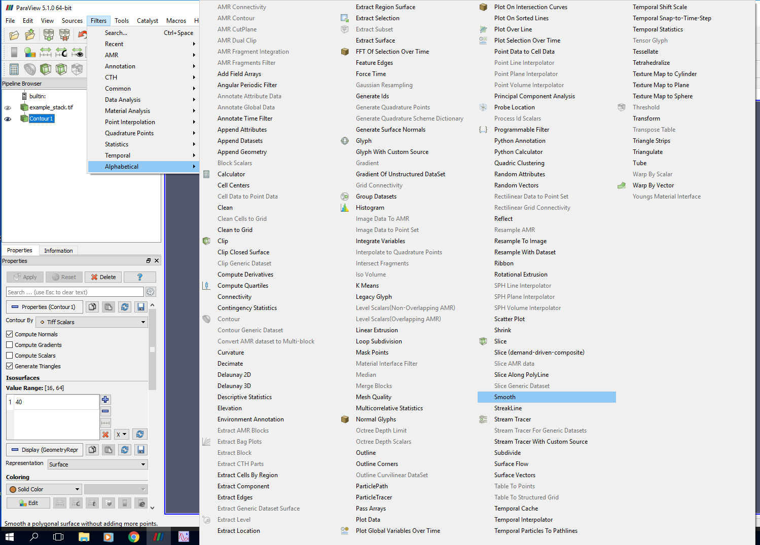
Fig.9 shows the Smooth function, in the Filters>Alphabetical tab
This will open the Smoothing tab in the properties tab, where the level of smoothing can be controlled by the number of iterations, as shown in Fig.10. The output of 2000 iterations of smoothing is also shown. It is worth noting that saving a surface as a .stl surface file will also apply some smoothing to the objects, this is covered in the ‘Mesh Generation – Iso2Mesh’ guide.
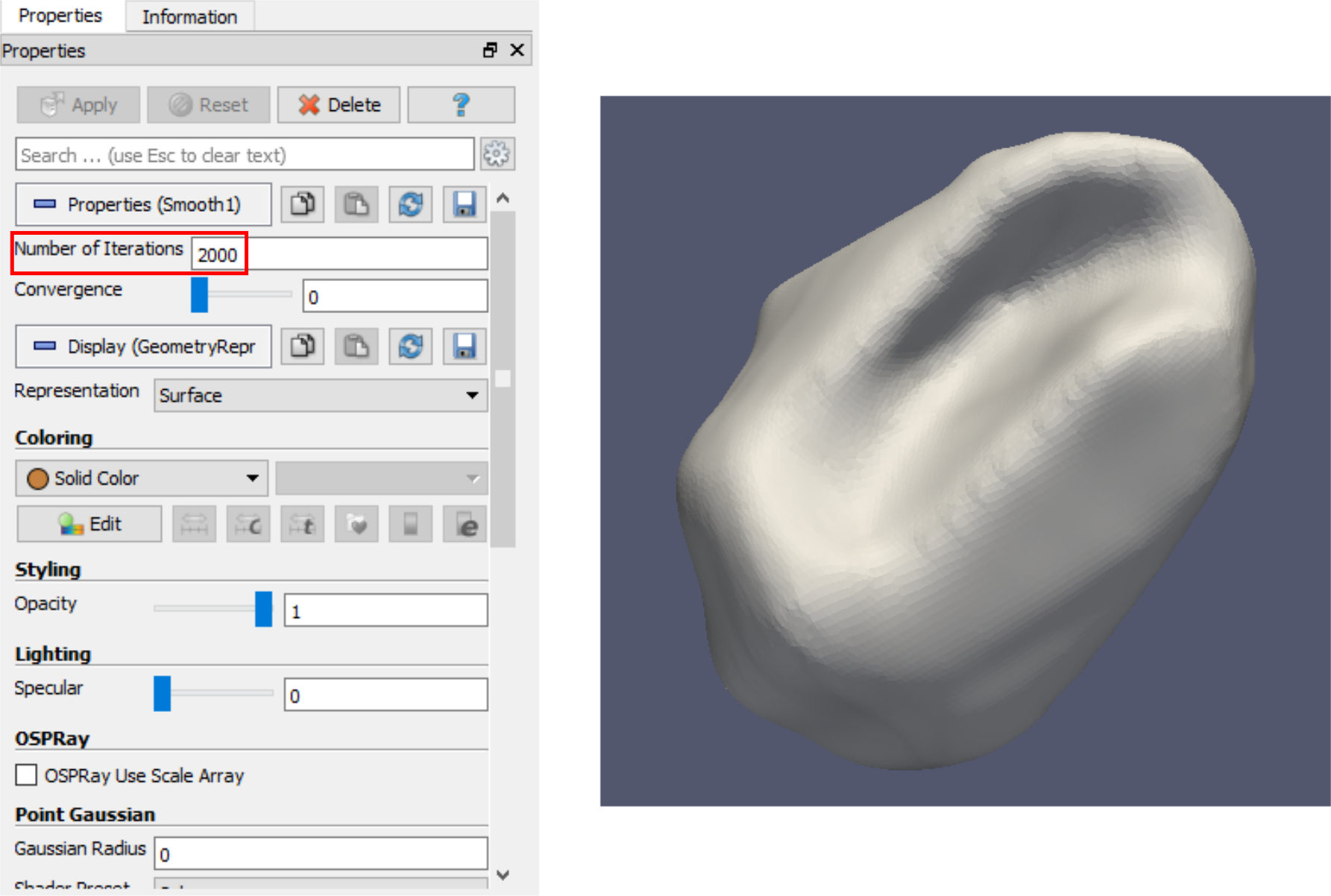
Fig.10 shows the Properties tab of the ‘Smooth’ function (left), with the Number of Iterations highlighted in red along with the output surface (right) after saving as a .stl file
Meshes
![]()
Opening and Visualising Meshes
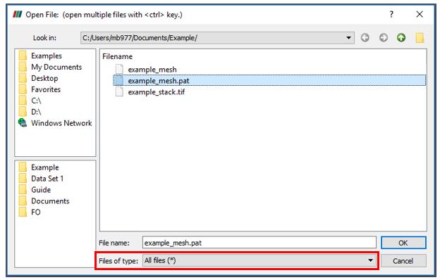
Fig.11 shows the Open File window, with the Files of type tab highlighted in red
Paraview can also be used to visualise tetrahedral meshes, once in a PATRAN format. Paraview does not recognise .pat extension files as true PATRAN files and so in order to open them, the ‘Files of type’ tab needs to be set to ‘All files (*)’ as shown in Fig.11. Once the .pat mesh has been selected the ‘Open Data With…’ prompt will open automatically, as shown in Fig.13. The ‘PATRAN Files’ option will then open the mesh file. The default representation will be a surface, but the mesh can also be viewed as a wiremesh using the ‘Wireframe’ option, which can be found in the ‘Representations’ tab, both options are shown in Fig.12.
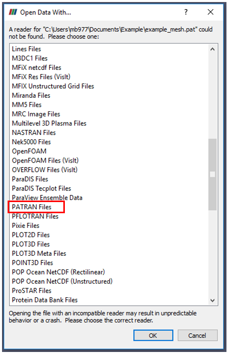
Fig.13 shows the Open Data With… window, with the PATRAN Files option highlighted in red
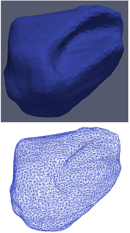
Fig.12 shows the example mesh shown as a surface (top), the default setting and as a wireframe (bottom)
Mesh Quality
Mesh quality can be very important, since very non equilateral tetrahedra can cause errors when running simulations in MERRILL. This can be checked in Paraview, using the ‘Mesh Quality’ function, which can be found in Filters->Alphabetical, as shown in Fig.14.
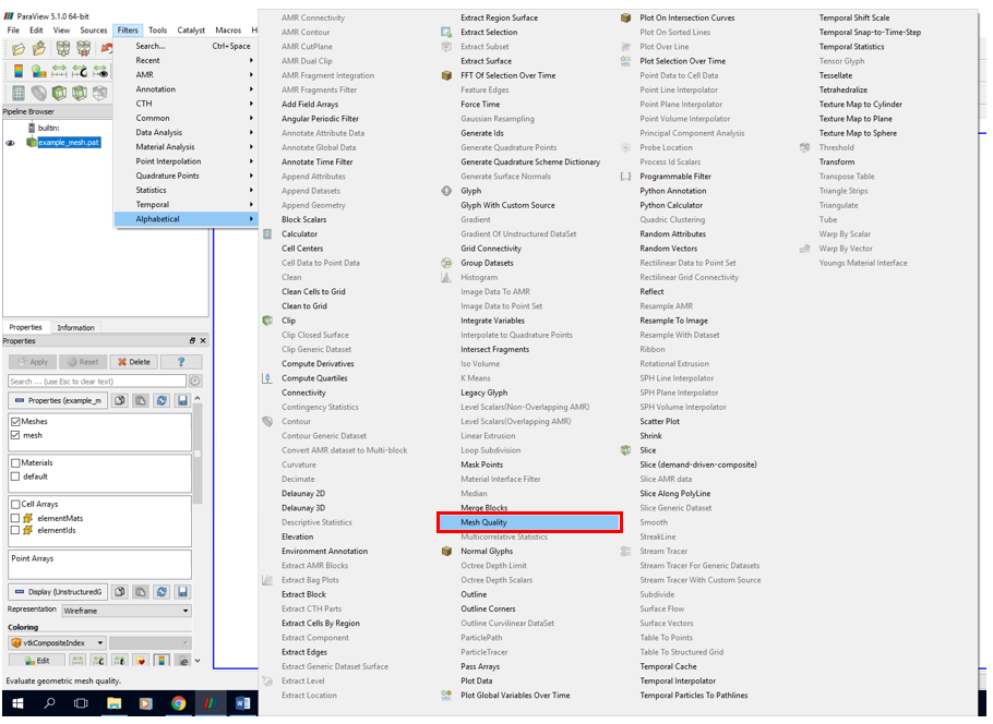
Fig.14 shows the Mesh Quality function, highlighted in red, and where it can be found in the Filters tab

Fig.15 shows the output of the mesh quality function on the example mesh
This function plots the tetrahedra on a scale from highest to lowest quality (blue to red respectively) as shown in Fig.15. Finding the lowest quality tetrahedra can be done using the ‘Threshold’ function, which can be found in Filters->Common. The lower bound of the threshold can then be set in the Properties tab as shown in Fig.16.
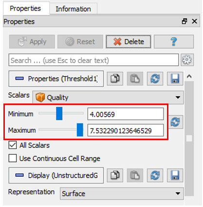
Fig.16 shows the Properties tab of the Threshold function, applied to a Mesh Quality output. Highlighted in red is the minimum and maximum level of the threshold
By setting the ‘Minimum’ value at the higher end of the quality range, the lowest quality tetrahedra can be isolated and viewed, as shown in Fig.17. Values below ~100 should cause no problems in MERRILL simulations, but values above may cause errors to occur and the meshes should be refined before use.
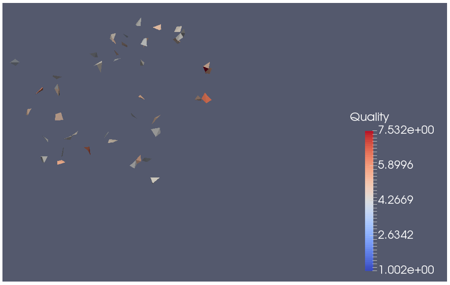
Fig.17 shows the output of the Threshold function applied to the Mesh Quality output of the example mesh, low quality tetrahedra can be seen in dark red
Simulations
Micromagnetic simulations using MERRILL produces .tec files of each of the magnetic states at each simulation step. These can be visualised in Paraview, allowing the individual steps in any simulation to be analysed, whether these steps are steps in external field, temperature or different random states.
These .tec files are loaded using the ‘Load State…’ function. This opens the ‘Load State File’ prompt. Here the ‘Takeshi X 0mT.pvsm’ should be chosen, not the .tec file. This loads the ‘Fix Paths in State File’ prompt. Selecting the ‘…’ icon will open another prompt. Here the .tec file is selected, these windows are shown in Fig.18. In the case that the simulation produces multiple .tec files, for example in a hysteresis simulation, these mult_tec files will appear as a single option here, selecting this will open all of the magnetic states, which can then be cycled through. Using the arrows at the top of the window.
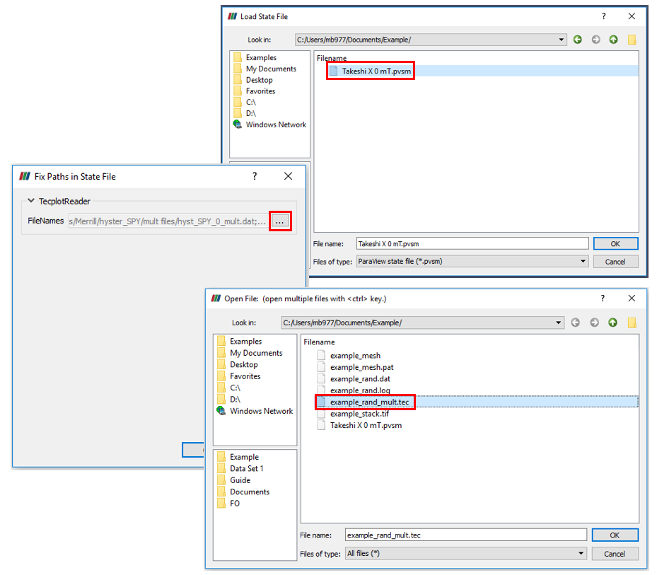
Fig.18 shows the three windows for opening a magnetic state. The Load State File window is shown upper right, with the Takeshi X 0mT.pvsm file highlighted in red. The Fix Paths in State File window is shown middle left, whilst the Open File window is shown bottom right, an example multi.tec file is highlighted in red
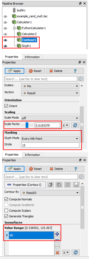
Fig.19 shows the Pipeline Browser with the two magnetic state objects, Contour1 and Glyph1, highlighted in red (top). The Properties tabs for both the Glyph1 (middle) and Contour1 (bottom) are also shown, with the editing options highlighted in red
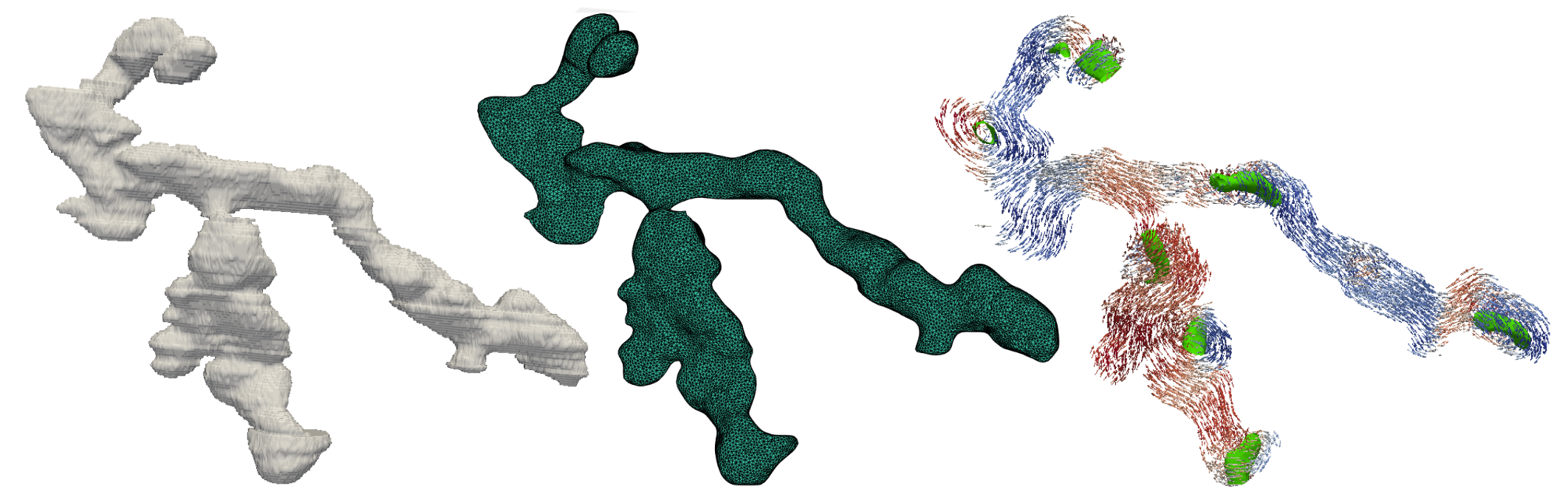
This will load the magnetic states into the objects shown in Fig.19. The two which can be used to control the visualisation are the ‘Contour1’ and ‘Glyph 1’ objects. The contour object is a surface which is taken at a specific level of helicity, and is used the show the core of magnetic vortices in the magnetic states. The glyph object contains the magnetic vectors. Both can be adjusted in the Properties tab. The example magnetic state before and after adjustment is shown in Fig.20. The density of the magnetic vectors and the size of the magnetic vectors can be changed using the ‘Glyph Mode’ and ‘Scale Factor’ options respectively. Changing the ‘Glyph Mode’ to ‘Every Nth Point’ and increasing the ‘Stride’ value reduces the number of vectors displayed, only every Nth vector, where N = ‘Stride’, is displayed. Lowering the value of the ‘Isosurfaces’ in the contour object Properties tab from the default value of 100 to a lower value, in this example 40, lowers the necessary helicity value at which a surface is created. The colour of the vectors is defined by their alignment along the Mx, My or Mz axis of the simulation, from negative to positive (blue to red).
![]()
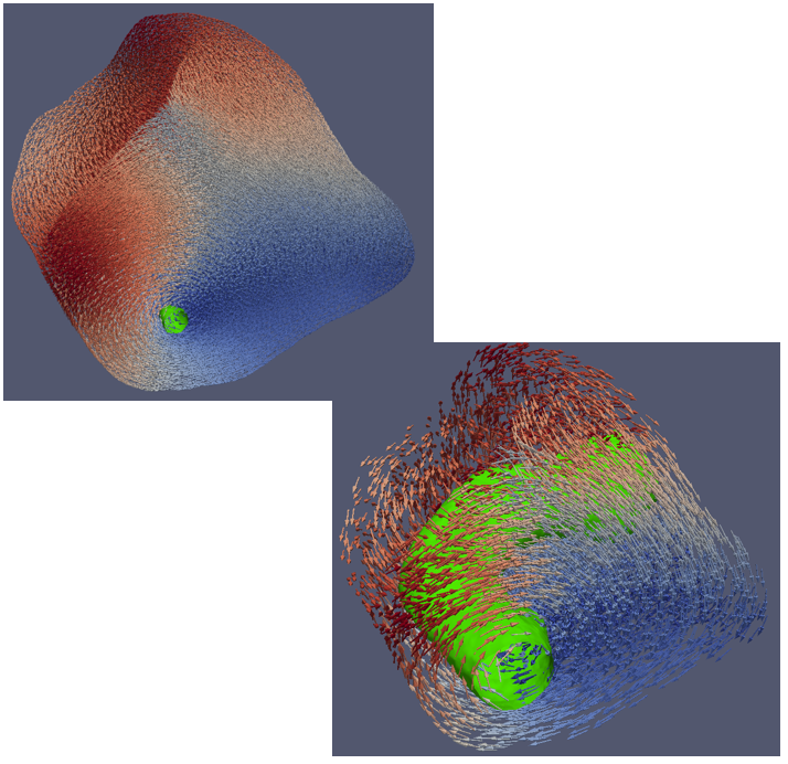
Fig.20 shows the example magnetic state before (above) and after (below) adjustment of the visualisation using the Contour1 and Glyph1 objects