Quick-Start Guide
ATHLETICS: Quick Start Guide
ATHLETICS works best when there is one set of micromagnetic data per IGOR Pro file. Once all the analysis has been performed, save the Igor Pro experiment under a new name, preserving the original file so it can be used for other simulations.
Note that the calculations can now consider both the magnetic and electronic contribution the electron beam phase shift. Holography images can be calulated with a mean inner potential contribution; see below. NOTE: there can be odd effects at surfaces if the mean inner potential is included. Lorentz calultions don’t include an electronic contribution as its effect is small and degraded image quality. However if you wish for it to be included in Lorentz images then please contact the author who can include it.
IGOR Pro requires that the file name of the data that are being loaded in does not exceed 28 characters in length including the file extension, does not start with a number and does not contain any punctuation marks other than spaces and underscores. NOTE: different versions of IGOR Pro operating on different platforms have different limits on file name character numbers. IOGR Pro 6.22A imposes the 28 character limit and earlier versions may require fewer characters. Try shortening input data file names if an error occurs – a start is to remove the file extension from the name, and then try renaming to shorten.
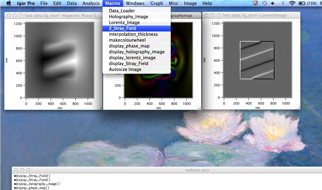
Below are the steps needed to produce images from the ATHLETICS script, and at the bottom there is an explanation of the features in the Macros tab. The images below correspond to to the test data from the Download page:
Step 1 Double Click the ATHLETICS icon to launch Igor Pro.
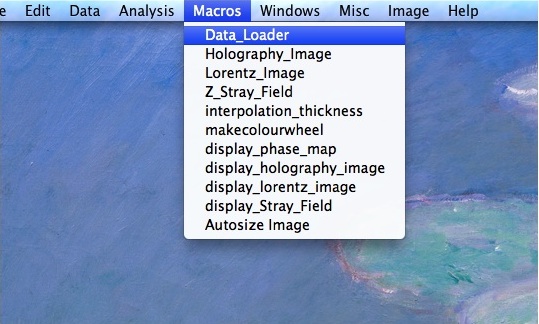
Step 2 Select Data_Loader from the Macros menu to load .txt or .llg_dom data
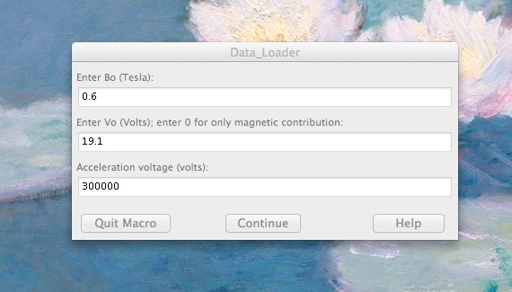
Step 3 Input the Bo and Vo value for your material, and the accelerating voltage corresponding to the microscope setting.

Step 4 Choose data of the form .txt or .llg_dom
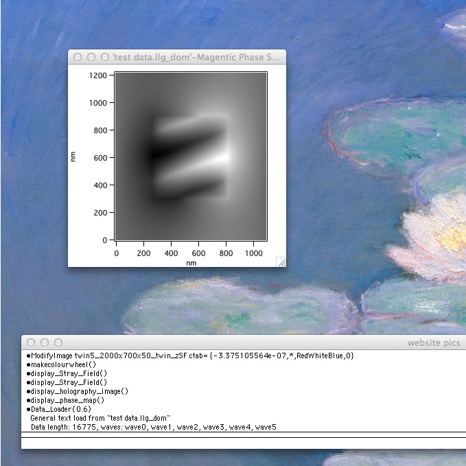
Step 5 A 2D phase map will appear of your input data averaged along the z direction and with empty space around the sample.
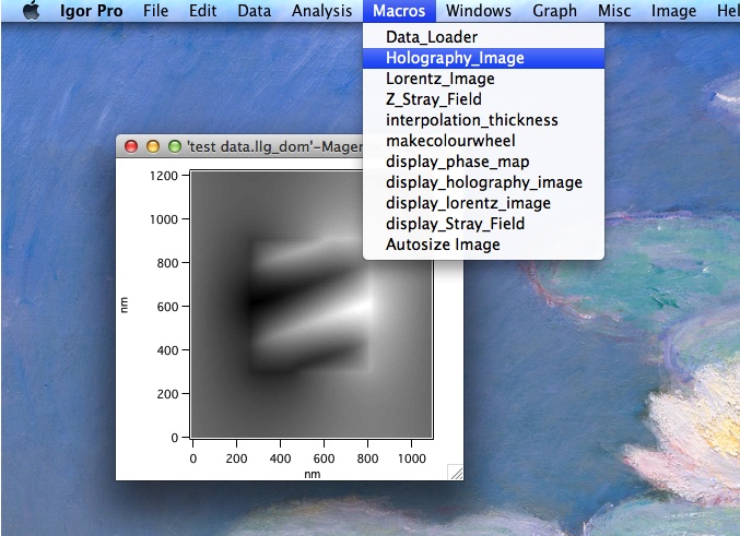
Step 6 To create an off-axis electron holography image, select Holography_Image from the macro menu
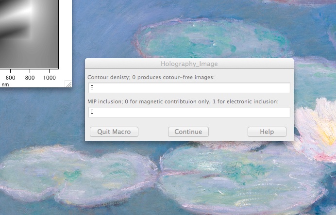
Step 7 Choose an holography density value; typically a value around 3 works well for a 50nm thick sample. Choose whether to include a mean inner potential in your holography image. A vlaue of 0 doesn’t include a mean inner potential (default), a value of 1 does include it.
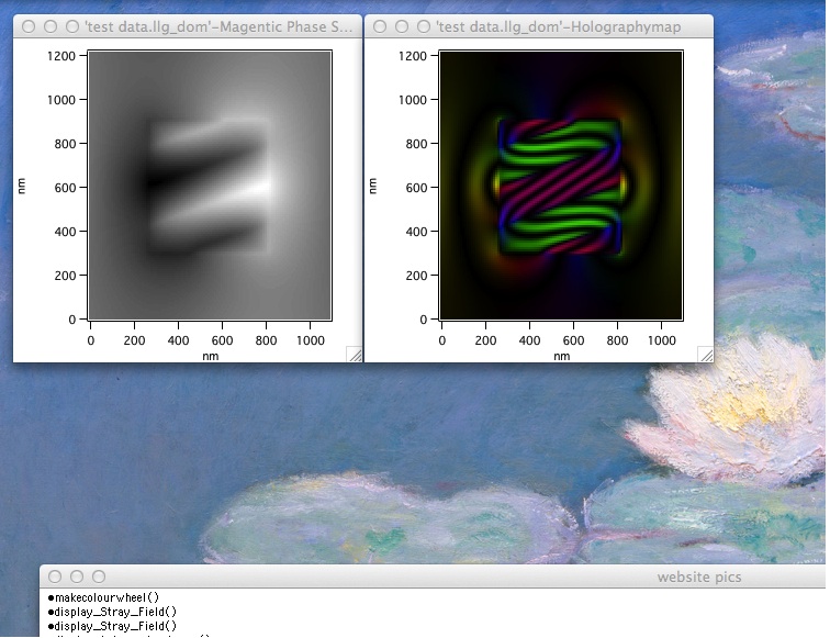
Step 8 An electron holography image will appear
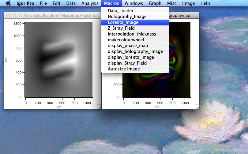
Step 9 To create a Lorentz contrast image select Lorentz_Image from the macro menu
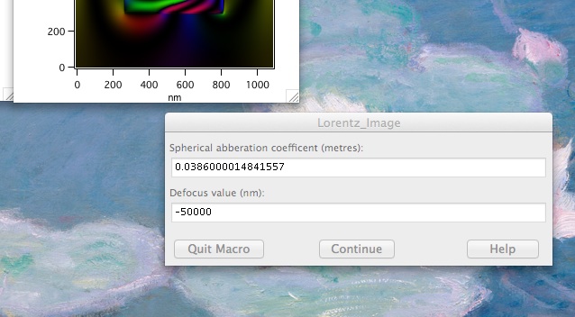
Step 10 Input microscope parameters to produce a Lorentz image; the parameters shown are only example parameters for this case
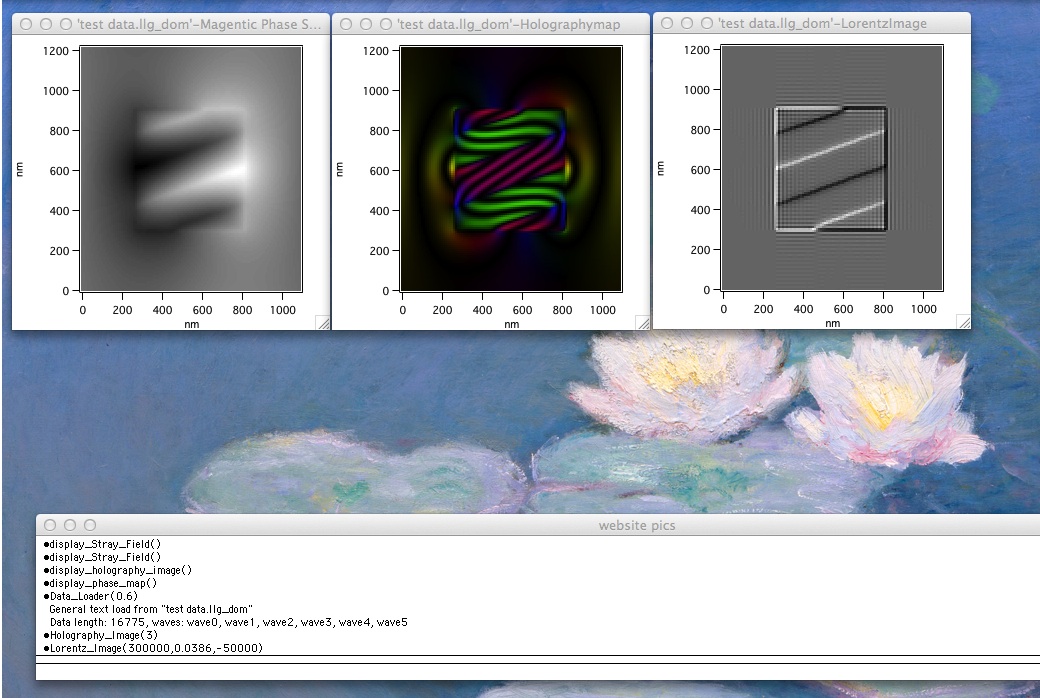
Step 11 A Lorentz contrast image will appear
Step 12 To create an out-of-plane stray field image select Z_Stray_Field from the macro menu
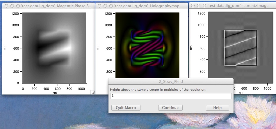
Step 13 Input the height above the sample to measure the stray field; this must be in integer multiples of the resolution e.g. if the resoltuion was 10nm then inputting a value of 1 would produce an image of the out-of-plane stray field at 10nm above the sample. The maximum value is 3 times the number of cells in the sample thickness (=thickness/resolution)
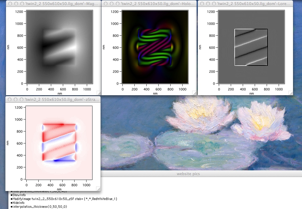
Step 14 An out-of-plane stray field image will be produced; red corresponds to positive, blue to negative and the colour intensity corresponds to magnitude
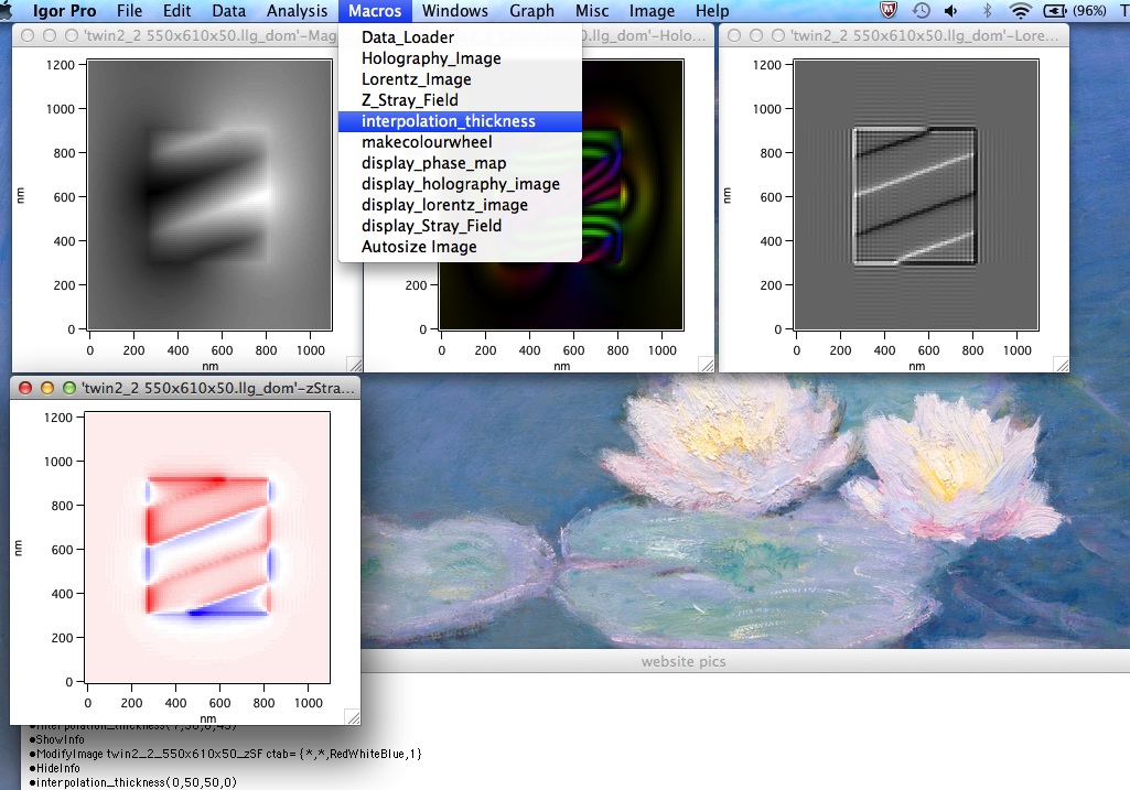
Step 15 To either interpolate the images to create smoother pictures, or add a constant thickness ramp to the images select interpolation_thickness from the macro menu.
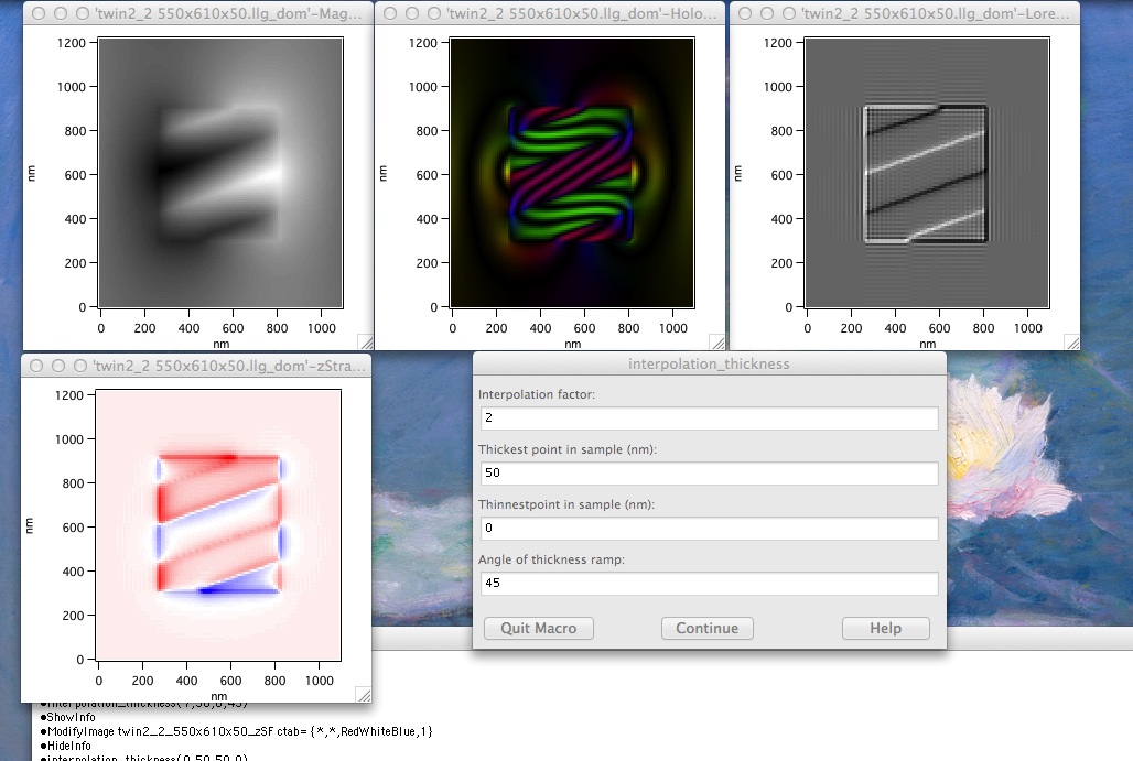
Step 16 Input an interpolation factor; about 2 produces noticeably clearer images. Input the thickest and thinnest points of the sample and the angle of change between these to add a thickness ramp. The thickest and thinnest points should correspond to the actual sample thickness and the angle of the ramp is in degrees from the positive y direction, between -180 and 180 degrees. An angle of 45 degrees here corresponds to a thickest point in the lower left corner and thinnest point in the upper right corner of the sample
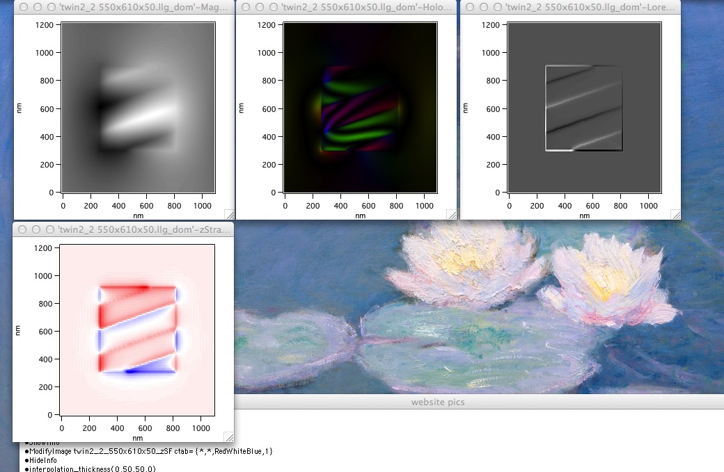
Step 17 An interpolated and thickness ramped phase map, holography image and Lorentz contrast image will appear. Note the fringes have gone from the Lorentz image and all images are less pixelated. Also note the effect of the thickness ramp where features get less intense as the sample gets thinner. The thickness ramp has no effect on the out-of-plane stray field images; see the the details of the interpolation_thickness macro below. To save any of these images, click on the image then select the ‘File’ tab and select ‘Save Graphics’
The Macros Menu:
Data_Loader: This is the first macro that should be run. Loads, manipulates and creates a phase map for .txt or .llg_dom files from LLG micromagnetic simulations. The sample is averaged along the z direction to create a 2D matrix, and then embedded in the center of a matrix that is twice as large as the sample in both directions. A phase map will appear to show that the data has been loaded properly. The phase map produced contains only the magnetic contribution to the phase shift. This must be the first macro that is run.
Holography_Image: creates and displays an off-axis electron holography image from the phase map calculated by data_loader. The program will ask for a contour density parameter – a value of around 3 works well for 50nm thick samples. This parameter can be altered to produce the best images. Entering 0 will produce contour-less images that still show the direction of the magnetic induction. To create an hologrphy image with the mean inner potential included put a value of 1 in the ‘MIP inclusion’ box; as a default this is set to zero which creates MIP-free images. NOTE: if the mean inner potential is included then there can be odd surface effects where contours can appear with extra curves.
Lorentz_Image: creates and displays a Fresnel-mode Lorentz contrast image from the phase map calculated by data_loader. The input parameters correspond to microscope settings. The values suggested are only examples that correspond to a common experiemental set up.
Z_Stray_Field: creates and displays the out-of-plane stray field at a defined height value above the sample from the data loaded in data_loader. The height value is in multiples of the resolution, so if the resolution of the micromagnetic simulation is 10nm then a value of 1 will produce an out-of-plane stray field image corresponding to 10nm above the sample. The maximum number of this value is 3 times the number of cells in the thickness, e.g. if a sample was 50nm thick with a 10nm resolution it is 5 cells thick, so the maximum value is 15, which corresponds to 150nm abve the sample. The minimum value is 1 and any integer between this and the maximum is acceptable.
Interpolation_thickness: Allows for images to be interpolated (so they appear smoother) and for the inclusion of a thickness ramp, between user defined thickest and thinnest points of the actual sample and an angle of change between these two. The angle should be inputted in degrees as a rotation from the positive y axis between -180 and 180 degrees i.e. 0 degrees corrosponds to the thickest point at the bottom of the image and the thinnest at the top and -90 degrees has the tickest point on the right and the thinnest on the left. N.B. Adding a thickness ramp doesn’t affect moment orientation, it just scales the phase; to see the effect of thickness changes on moment orientations the micromagentic simulations need to be re-run with thickness changes included. Interpolating slows simulations so it is advised that, if other parameters are to be changed first, the interpolation paramater is the last to be changed to save time. A value of 2 shows clear improvment to images, but larger values can be chosen if so wished. The default interpolation value is 1 and the default ramp is a flat sample at the thickness deduced from the inputted data. The new interpolated or thickness ramped images will replace the ones already produced. This macro has no effect on the out-of-plane stray field image as these images are designed with quantitative analysis in mind and interpolating will affect values. For quantitative Lorentz analysis images shouldn’t be iterpolated. This macro can not be run before both holography_image and lorentz_image have been run – an error message will appear if this attempted.
Makecolourwheel: Displays a colour wheel corresponding to previously published experimental holography results. If a colour wheel is already displayed running this macro will move it so it is the front window.
Display_Phase_map: Displays a copy of the phase map with the most recently inputted interpolation and thickness ramp values. Running this macro (whether there is a phase map displayed or not) will always produce a phase map. This macro only works once data_loader has been run.
Display_holography_image: This macro is designed to display a copy of the holography image with the parameters that have most recently been inputted into holography_image and interpolation_thickness (whether there is an holography image displayed or not). If this macro is run before holography_image has been, then this macro will run holography_image asking for parameters to be entered, and an image will be produced. After holography_image has been run this macro will only produce copies of the holography image, and no longer asks for parameters. To change the parametrs use holography_image and interpolation_thickness.
Display_Lorentz_image: This macro is designed to display a copy of the Lorentz image with the parameters that have most recently been inputted into lorentz_image and interpolation_thickness (whether there is a Lorentz image displayed or not). If this macro is run before lorentz_image, then this macro will run lorentz_image asking for parameters to be entered, and an image will be produced. After lorentz_image has been run this macro will only produce copies of the Lorentz image, and no longer asks for parameters. To change the parametrs use lorentz_image and interpolation_thickness.
Display_Stray_field: This macro is designed to display a copy of the out-of-plane stary field image with the parameters that have most recently been inputted into z_stray_field and interpolation_thickness (whether there is an out-of-plane stray field image displayed or not). If this macro is run before z_stray_field, then this macro will run z_stray_field asking for parameters to be entered, and an image will be produced. After z_stray_field has been run this macro will only produce copies of the out-of-plane stary field image, and no longer asks for parameters. To change the parametrs use z_stray_field and interpolation_thickness.