
FORCem
*** New ***
FORCem now integrated with FORCinel 3.0!
Download FORCinel
1. Overview
FORCem (FORC environmental magnetism) is a program designed to automatically upload and analyze a suite of raw FORC files that have been measured using identical experimental protocols. The analysis permits the quantification of the FORC assemblage end member proportions using a method based on principal component analysis.
FORCem is written by Ioan Lascu and Richard Harrison of the Department of Earth Sciences, University of Cambridge. Please feel free to contact the authors with any questions/bug reports/feature requests, or leave a note in the comments section.
FORCem is free to use, but please cite the article outlining the methodology in any scientific publications that use the software:
Lascu, I., Harrison, R. J., Li, Y. T., Muraszko, J. R., Channell, J. E. T., Piotrowsky, A. M. and Hodell, D. A., 2015, Magnetic Unmixing of First-Order Reversal Curve Diagrams using Principal Component Analysis. Geochemistry, Geophysics, Geosystems 16, doi: .
2. Download
With the release of FORCinel 3.0, FORCem has now been fully integrated into the main FORCinel package. To download FORCinel 3.0 go to our Download FORCinel site.
We will provide an updated set of instructions and a video tutorial explaining how to run FORCem within FORCinel 3.0 as soon as possible. For now, you may still find the instructions for the original version of FORCem (which can be downloaded using the link below) useful.
This file contains the original FORCem, along with a pre-loaded data set (from core SHAK-10-9M-F collected from the Iberian Continental Margin) and can be readily used to test the PCA-based unmixing method (i.e., skip section 4.1. and go directly to section 4.2. below).
3. System Requirements
FORCem is a self-contained package written using Igor Pro by WaveMetrics. Although Igor Pro is a commercial package, a fully functioning demo version can be downloaded for free for Mac and Windows. This will allow you to explore FORCem, but will not allow you to export results after 30 days.
FORCem has been written using Igor Pro version 6.36, on a Mac Mini with a 2.6 GHz Intel Core i7 processor and 16 GB RAM, running OS X version 10.8.5. The program has also been tested successfully on a MacBook Pro with a 2.2 GHz Intel Quad Core i7 processor and 4 GB RAM. We cannot be guarantee full functionality on other systems using different software versions, so do get in touch if you run into trouble.
4. Running FORCem
Before using FORCem, it is recommended that one or more samples be analyzed using FORCinel to determine optimal parameters for smoothing, ridge extraction, grid definition, etc. These parameters should then be used on the entire dataset when running FORCem.
After downloading and unzipping the file FORCem.pxp, simply double click to open it within Igor Pro. You should see the following windows in addition to the ‘FORCem’ command window:
- ‘Data Browser’
- ‘FORC Control Panel’
- ‘PCA Control’
- ‘Define Endmembers’
If not all the windows are visible on your screen, go to the menu bar and click Windows>Control>Retrieve All Windows in order to move them into visible positions.
4.1. Loading FORCs
To load the suite of raw FORC files, press ‘Load multiple FORCs’ in the FORC Control Panel. (Note that in Igor, before pressing a panel button, the respective window needs to be selected.) The ensuing dialog window asks for the folder containing the raw FORC files to be analyzed. All the files should have an extension (e.g., *.frc), as the next dialog box asks for this extension name (‘frc’ in this case). Be aware that data from all the files with the specified extension in the selected folder will be uploaded.
The user is then prompted to choose whether certain actions should be performed, or to input some processing parameters. The succession of dialog boxes contains the following operations:
- Perform drift correction
- Remove first point artefact
- Remove lower branch
- Input VARIFORC smoothing parameters
- Indicate wave name containing sample masses (optional)
- Extract central ridge
All of the above are standard FORCinel 2.0 operations, except for item 5. If used, the wave containing the sample masses should be created or imported in the Results folder (see Data Browser window).
Depending on the size and number of data files, the uploading and processing of the FORC data may take several hours (to get a rough estimate multiply the total processing time of one data file in FORCinel by the number of files to upload).
The upload procedure will create a series of waves in Results, among which is a 3D wave called totalstack, in which each layer will contain one processed FORC diagram (the equivalent of the wave variforc_raw in FORCinel). This wave will be used in the PCA.
4.2. PCA Procedures
Once the data are uploaded (or if using the preloaded data in FORCem_demo.pxp), press ‘PCA Grid’ in the PCA Control window, and input the grid dimensions (in T). For typical magnetite-bearing samples a resampling resolution of 0.005 T is recommended for short processing times. A resolution of 0.002 T can be employed for small grids (0.1 x 0.1 T). For higher coercivity minerals a resolution >0.005 T is recommended.
The individual grids are redimensioned and placed into a wave called Dat_matrix, in which each line is an unfolded grid presented as a succession of vertical profiles (the so-called PCA spectrum). The subtraction of the mean PCA spectrum produces the wave meanmatrix, which will be used in the PCA. Both Dat_matrix and meanmatrix are plotted at the end of the gridding procedure.
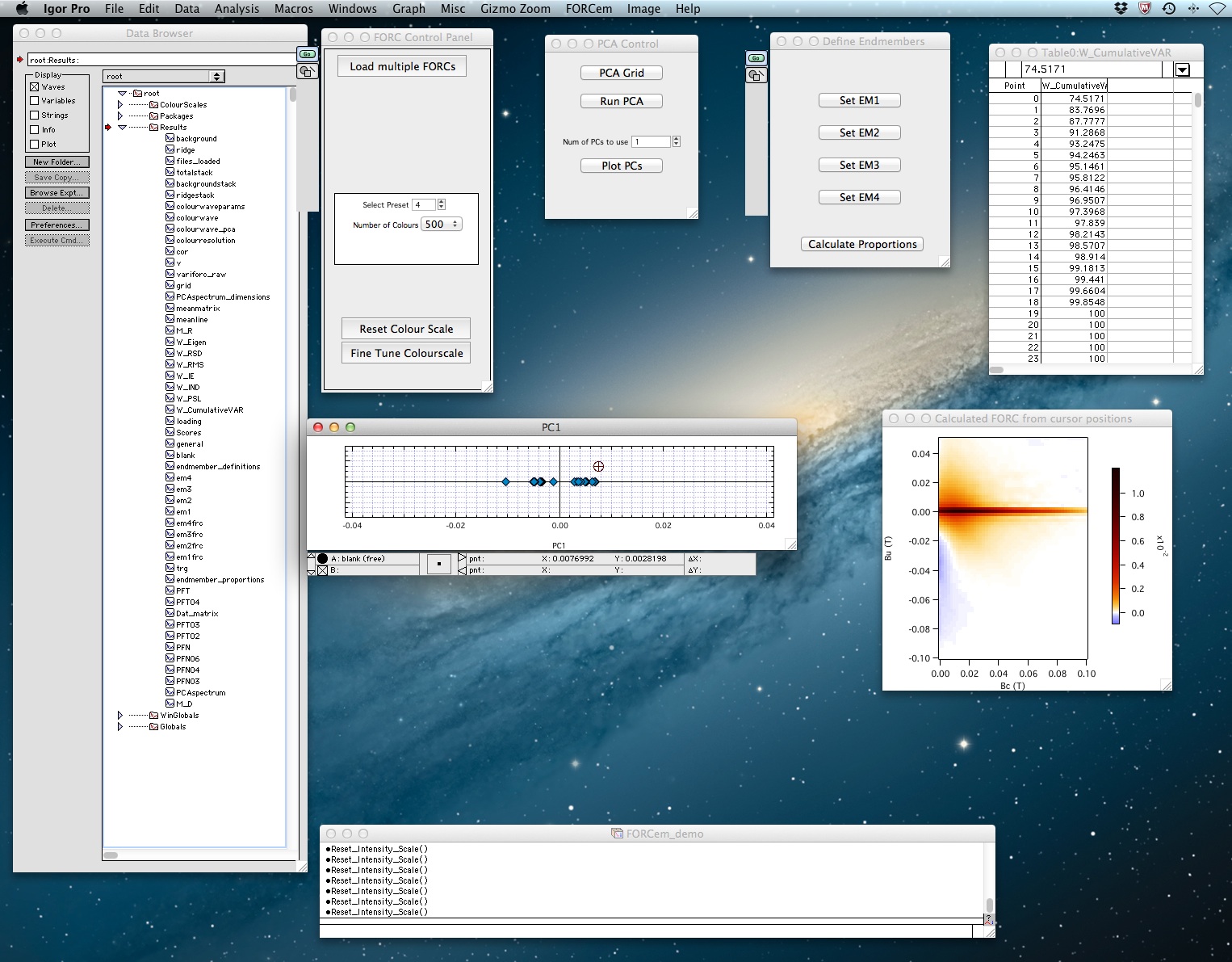
To perform the PCA press ‘Run PCA’ in the PCA Control window. The end of the run (which can last for a few minutes if meanmatrix is large) is signaled by the display of a table containing the cumulative variances of the PCs. The next step is to select ‘num of PCs to use’ in the PCA Control window. The number of PCs used is subject to user interpretation of the dataset and of the values in the displayed table. The software currently accepts values of 1, 2, or 3, corresponding respectively to binary, ternary, and quaternary mixtures.
After selecting the number of significant PCs, press ‘Plot PCs’ in the PCA Control window to display the PC score plot(s) and a general FORC diagram calculated using user-defined PC scores values. These PC scores are controlled by a moveable cursor (⊕) within the score plot. After selecting the score plot window, move the cursor either by using the arrow keys, or by clicking and dragging it to the desired position. The FORC diagram will be automatically updated.
4.3. Selecting End Members and Calculating Proportions
If there is only one significant PC, all the data points can be expressed as linear combinations of two end members (EMs) with PC 1 values outside the interval spanned by the data. The cursor movement in the score plot (titled ‘PC1’) will only relay values in the horizontal direction. Move the cursor beyond the data interval in one direction until a physically realistic EM FORC geometry is attained (axes and colors can be rescaled if necessary). Select the Define Endmembers window and press ‘Set EM1’. A table called End Member PCs containing EM score values will be displayed. Select the score plot and move the cursor beyond the data interval in the opposite direction until a second suitable EM is obtained. Select the Define Endmembers window and click ‘Set EM2’, making sure that the score value has registered in the table. Then press ‘Calculate Proportions’. A graph with proportion values for each EM will be displayed, along with calculated FORC diagrams for each EM.
If there are two significant PCs, the data points can be expressed as linear combinations of three EMs. The cursor in the score plot (titled ‘PC1 and PC2’) will register score values for both PC 1 and PC 2, which will be used to calculate the general FORC diagram. Apply the same procedure described above to select and display the three end members. After calculating proportions, a red triangle will be displayed in the score plot. Check that all non-outlying data points are contained within this triangle. If necessary adjust EMs and recalculate proportions. In addition to the proportions graph, one can plot this triangle as a ternary diagram, by going to the menu and clicking Windows>New>New Ternary Diagram, and then selecting the A, B, and C components as the waves em1, em2, and em3 found in the Results folder. The value in the box labeled ‘Select Z Data (for Contour Plot)’ can be left as “_none_”.
If there are three significant PCs, the data points can be expressed as linear combinations of four EMs. In addition to the PC2 vs. PC1 score plot and the general FORC diagram, a PC3 vs. PC1 score plot and a 3D plot of the score space will be displayed. These additional graphs are intended to help better visualize the three dimensional score space and assist with EM selection. The second score plot contains a cursor that controls PC 3 score values, which can only be moved in the vertical direction. The cursor moves automatically in the horizontal direction when moving the cursor in the first score plot. PC 3 values can also be controlled by manually changing the value in the PC3 box that now appears in the PC2 vs. PC1 score plot. After settling on suitable EMs and calculating proportions, the 3D score plot will be updated with a triangular pyramid whose vertices are the four EMs. Projections of this pyramid will appear in the 2D score plots. Check that all non-outlying data points are contained within this pyramid. An additional 3D plot of the quaternary mixing diagram is displayed. In this case the pyramid is a regular tetrahedron, with the data points situated at proportional distances from the vertices.
N.B. If experimenting with different scenarios for the number of significant PCs (i.e., if you want change the value for ‘Num of PCs to use’), it is recommended to close all windows (except the initial 5 windows and the cumulative variance table) before pressing ‘Plot PCs’.
5. Video Demo of FORCem
Here is a useful demonstration of how to use FORCem. The video is a fragment of a lecture on FORC processing held by Richard Harrison at the University of Minnesota FORC Workshop in July 2015. The entire talk (which includes a comprehensive demo of FORCinel) can be found at the University of Minnesota Digital Conservancy.
Harrison, Richard (2015). Simple and Advanced Processing of FORC Data. Retrieved from the University of Minnesota Digital Conservancy. http://hdl.handle.net/11299/173973.
5 Responses to FORCem
- Pingback:Pengfei Liu
- Pingback:Richard Harrison
- Pingback:Richard Harrison
- Pingback:Yang Xiaoqiang
- Pingback:Richard Harrison
- Pingback:Richard Harrison
- Pingback:chhavi
Leave a Reply